Hi @nvar . Very interesting question! We should explain this better in the tutorial (or elsewhere). The reason why we replace the “standard” STDP equations by differential equations in the tutorial is that it models “all-to-all” interactions, i.e. a spike triggers updates depending on its distance in time to all preceding spikes – of course, most of them happened sufficiently long ago that they won’t have any effect in practice. In equations, this is usually expressed with some “sum over previous spike times” term. This would be very inefficient to implement directly (need to store all previous spike times, need to run a sum over more and more terms or need to introduce some cut-off, etc.), but can be implemented in a straightforward and efficient way with the differential equation formalism. In your paper, this is not necessary, since they are using a “nearest-neighbor” implementation, i.e. for each spike we are only interested in its interaction with the preceding spike. You can recognize these models by the absence of a “sum over spike times” term, and by formulations like "\delta t_{ij} is the difference between the presynaptic spike time t_i and the postsynaptic spike time t_j" (i.e., there is only a single pre- and postsynaptic spike time to consider). You can find more about this topic in section 4.1.2 of Morrison et al. (2008).
Since we only have to consider a single spike time for each pre- and postsynaptic neuron, we can store this time for each spike as a variable in the neuron, and then refer to it with the equation directly copied from the paper. If your neuron model uses refractoriness, Brian automatically defines a lastspike variable. If not, you can add it to the equations yourself, and update it for every spike.
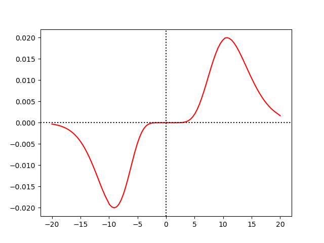
Below, example code that does this. Instead of a real neuron model, it uses a neuron that simply spikes at a predetermined time. One neuron spikes at 30ms, and 100 neurons spike at times between 10ms and 50ms. By connecting the first neuron to all the other neurons, we get pre/post pairings with \delta t_{ij} values between -20ms and 20ms. For each pre- and post-synaptic spike, we then store the spike time in the lastspike variable of the respective neuron, calculate \delta t_{ij}, and then update w according to the equation you posted (using two different \alpha variables for positive and negative \delta t_{ij} values, i.e. pre-before-post and post-before-pre pairings):
from brian2 import *

beta = 10.0
alpha_pre_post = 0.94  # delta_t > 0
alpha_post_pre = 1.1   # delta_t < 0
g_0 = 0.02
g_norm = beta**beta * exp(-beta)

G = NeuronGroup(101, '''
spike_when : second (constant)
lastspike : second  # remove when model uses refractory
''',
threshold='timestep(t, dt) == timestep(spike_when, dt)') # spike at pre-defined time
G.lastspike = -1e9*second
G.spike_when[0] = 30*ms
G.spike_when[1:] = np.linspace(10, 50, 100)*ms

S = Synapses(G, G, 'w : 1',
on_pre='''
lastspike_pre = t
delta_t = (lastspike_post - lastspike_pre)/ms
w += g_0/g_norm * alpha_post_pre**beta*abs(delta_t)*delta_t**(beta - 1)*exp(-alpha_post_pre*abs(delta_t))
''',
on_post='''
lastspike_post = t
delta_t = (lastspike_post - lastspike_pre)/ms
w += g_0/g_norm * alpha_pre_post**beta*abs(delta_t)*delta_t**(beta - 1)*exp(-alpha_pre_post*abs(delta_t))
''',
)
S.connect(i=0, j=np.arange(1, 101))  # Connect first neuron to all other neurons

run(51*ms)

plt.plot((G.spike_when[1:] - G.spike_when[0])/ms, S.w[:], color='r')
plt.axhline(linestyle=':', color='k')
plt.axvline(linestyle=':', color='k')
plt.show()
The result seems to faithfully reproduce their curve (the value on the y axis goes up to \pm g_0 instead of \pm 1, but they probably normalized things for the plot.