Description of problem
I’m trying to make the neuronal population fire according to precomputed sequences of firing. An encoding scheme produces those firing sequences. For instance, let’s assume i have 100 neurons
at t = 0 to 100 ms
[1, 20,12,23, ….. 67] —– fires at [0,1,2,5,6,11,…..]
at 100ms to 200ms
[2,1,55,3,8,90,1………] —–fires at [0,3,5,6,………..]
at 200ms to 300ms
………
It fires all neuronal populations at different times within a 100-ms period for the entire simulation, which lasts 10 seconds.
Minimal code to reproduce the problem
from brian2 import *
import os
import matplotlib.pyplot as plt
import numpy as np
taue = 5*ms
taui = 10*ms
Ee = 0*mV
Ei = -70*mV
os.environ['CC'] = 'gcc'
os.environ['CXX'] = 'g++'
dimension = 18
#t = 100
nGRFcells = 5
gamma = np.ones((nGRFcells, dimension))
Imax = np.max(info_matrix, axis = 0)
Imin = np.min(info_matrix , axis = 0)
print("I max", Imax)
print("I min", Imin)
iterations = 10
G = SpikeGeneratorGroup( dimension * nGRFcells, indicess, firing_t*ms)
# taken from Touboul_Brette_2008
eqs = """
dvm/dt = (g_l*(e_l - vm) + g_l*d_t*exp((vm-v_t)/d_t) + I_AMPA - I_NMDA + I_GABA +- w)/c_m : volt
dw/dt = (a*(vm - e_l) - w)/tau_w : amp
I_AMPA = ge * (Ee - vm): amp
I_GABA = gi * (Ei - vm): amp
dge/dt = -ge / taue : siemens
dgi/dt = -gi / taui : siemens
I_NMDA: amp
"""
taum = 20*ms
taupre = 200*ms
taupost = 180*ms
gmax = .1
dApre = .0002
dApost = -dApre * taupre / taupost * 1.05
dApost *= gmax
dApre *= gmax
patterns = {
"tonic spiking": {
"c_m": 200 * pF,
"g_l": 10 * nS,
"e_l": -70.0 * mV,
"v_t": -50.0 * mV,
"d_t": 2.0 * mV,
"a": 2.0 * nS,
"tau_w": 30.0 * ms,
"b": 0.0 * pA,
"v_r": -58.0 * mV,
"i_stim": 500 * pA,
},
"adaptation": {
"c_m": 200 * pF,
"g_l": 12 * nS,
"e_l": -70.0 * mV,
"v_t": -50.0 * mV,
"d_t": 2.0 * mV,
"a": 2.0 * nS,
"tau_w": 300.0 * ms,
"b": 60.0 * pA,
"v_r": -58.0 * mV,
"i_stim": 500 * pA,
},
"initial burst": {
"c_m": 130 * pF,
"g_l": 18 * nS,
"e_l": -58.0 * mV,
"v_t": -50.0 * mV,
"d_t": 2.0 * mV,
"a": 4.0 * nS,
"tau_w": 150.0 * ms,
"b": 120.0 * pA,
"v_r": -50.0 * mV,
"i_stim": 400 * pA,
},
"regular bursting": {
"c_m": 200 * pF,
"g_l": 10 * nS,
"e_l": -58.0 * mV,
"v_t": -50.0 * mV,
"d_t": 2.0 * mV,
"a": 2.0 * nS,
"tau_w": 120.0 * ms,
"b": 100.0 * pA,
"v_r": -46.0 * mV,
"i_stim": 210 * pA,
},
"delayed accelerating": {
"c_m": 200 * pF,
"g_l": 12 * nS,
"e_l": -70.0 * mV,
"v_t": -50.0 * mV,
"d_t": 2.0 * mV,
"a": -10.0 * nS,
"tau_w": 300.0 * ms,
"b": 0.0 * pA,
"v_r": -58.0 * mV,
"i_stim": 300 * pA,
},
"delayed regular bursting": {
"c_m": 100 * pF,
"g_l": 10 * nS,
"e_l": -65.0 * mV,
"v_t": -50.0 * mV,
"d_t": 2.0 * mV,
"a": -10.0 * nS,
"tau_w": 90.0 * ms,
"b": 30.0 * pA,
"v_r": -47.0 * mV,
"i_stim": 110 * pA,
},
"transient spiking": {
"c_m": 100 * pF,
"g_l": 10 * nS,
"e_l": -65.0 * mV,
"v_t": -50.0 * mV,
"d_t": 2.0 * mV,
"a": 10.0 * nS,
"tau_w": 90.0 * ms,
"b": 100.0 * pA,
"v_r": -47.0 * mV,
"i_stim": 180 * pA,
},
"irregular spiking": {
"c_m": 100 * pF,
"g_l": 12 * nS,
"e_l": -60.0 * mV,
"v_t": -50.0 * mV,
"d_t": 2.0 * mV,
"a": -11.0 * nS,
"tau_w": 130.0 * ms,
"b": 30.0 * pA,
"v_r": -48.0 * mV,
"i_stim": 160 * pA,
},
}
L1parameters = patterns["irregular spiking"]
L2parameters = patterns["adaptation"]
neuron = NeuronGroup(
100,
model=eqs,
threshold="vm > 0*mV",
reset="vm = v_r; w += b",
method="euler",
namespace=L1parameters,
)
neuron.vm = L1parameters["e_l"]
neuron.w = 0
# connecting the Cortical layer into output layer L4
#So = Synapses(G,neuron, on_pre='ge += 10*nS')
#So.connect(p=0.05)
S = Synapses(G, neuron,
'''w1 : 1
dApre/dt = -Apre / taupre : 1 (event-driven)
dApost/dt = -Apost / taupost : 1 (event-driven)''',
on_pre='''ge += w1 * siemens
Apre += dApre
w1 = clip(w1 + Apost, 0, gmax)''',
on_post='''Apost += dApost
w1 = clip(w1 + Apre, 0, gmax)''',
)
S.connect(p = 0.05)
S.w1 = '0.0001* rand()'
s = []
L1_mon = SpikeMonitor(neuron)
spike_mon = SpikeMonitor(G)
w_mon = StateMonitor(S, 'w1', record=[0,1,2])
net = Network(G,neuron,S,L1_mon,w_mon, spike_mon)
for iter1 in range(iterations):
index = np.random.randint(10) # index for the active neuron
s.append(index)
print("index",index)
y = np.array(attributes[index][2])
indicess, firing_t = encoding_layer(y,Imin, Imax, dimension, 100, gamma , nGRF = nGRFcells)
net.run(100 * ms)
G.set_spikes(indicess, firing_t * ms + 100 * (iter1 + 1) * ms)
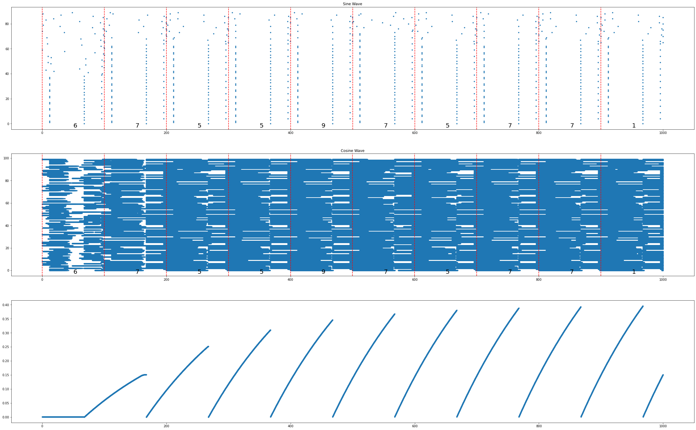
# Create a figure
plt.figure(figsize=(40, 25))
# Create the first subplot (1 row, 2 columns, 1st subplot)
plt.subplot(3, 1, 1)
plt.plot(spike_mon.t/ms, spike_mon.i, '.')
plt.title('Sine Wave')
for l in range(0,1000, 100):
plt.axvline(l, ls='--', c='r')
# add text, s to a point at (x, y) coordinate in a plot
idx = int(l/100)
plt.text(l+50 , -3, str(s[idx]),fontsize=20)
# Create the second subplot (1 row, 2 columns, 2nd subplot)
plt.subplot(3, 1, 2)
plt.plot(L1_mon.t/ms, L1_mon.i, '.')
plt.title('Cosine Wave')
for l in range(0,1000, 100):
plt.axvline(l, ls='--', c='r')
# add text, s to a point at (x, y) coordinate in a plot
idx = int(l/100)
plt.text(l+50 , -3, str(s[idx]),fontsize=20)
plt.subplot(3,1,3)
plt.plot(w_mon.t/ms, w_mon.w1[0]/gmax, '.')
# Adjust layout for better spacing
#plt.tight_layout()
plt.show()
What have you already tried
i have tried to use SpikeGeneratorGroup with set_spikes function in for loop, it works but it seems the weights are reinitalized every time i run the simulation within the loop.
Expected output (if relevant)
Actual output (if relevant)
I’m expecting Brian2 to retain the parameter values from the last run and update them without resetting them. The purpose is to run all of these sets of indices and times within one simulation a 100ms window.