Pinsky Rinzel - spiking problem

[imlittledove]

Description of problem

Hello everyone! I’m trying to build a single neuron model with the Pinsky Rinzel model of 1994. Even though I’m producing graphs i cannot seem to produce spikes. I’m really hoping someone can identify the problem and point out what i should do to proceed forward.
Thank you in advance everyone
the paper for reference:

1. Intrinsic and Network Rhythmogenesis in a Reduced Traub Model
   for CA3 Neurons (Pinsky and Rinzel, 1994).

Also since i’m a new user i’m not allowed to put more than one embedded items so i will only attach the code and when you reproduce it you will get the plots as well

Minimal code to reproduce problem

#%%
from brian2 import *
import matplotlib.pyplot as plt
start_scope()

defaultclock.dt = 0.05 * ms

Parameters = {
    'C_s': 1* uF / cm ** 2,
    'C_d': 1 * uF / cm ** 2,
    'I_s': 0.75 * uA/ cm ** 2,
    'I_d': 0 * uA/ cm ** 2 ,
    'v_s': -65*mV,
    'v_d': -65*mV,
    'g_Na': 30 * msiemens / cm ** 2,
    'E_Na': 115 * mV,
    'g_Kdr': 15 * msiemens / cm ** 2,
    'E_K': -15 * mV,
    'g_L': 0 * msiemens / cm ** 2,  # leak
    'E_L': 0 * mV,
    'g_Ca': 10 * msiemens / cm ** 2,
    'E_Ca': 80 * mV,
    'g_Kahp': 0.8 * msiemens / cm ** 2,
    'g_KC': 15 * msiemens / cm ** 2,
    'g_Abeta': 0 * msiemens / cm ** 2,
    'E_Abeta': -65 * mV,
    'g_c': 2.1 * msiemens / cm ** 2,
    'p': 0.5,

}

eqs = '''
#membrane potential
#soma:
dv_s/dt=(- ILs -INa - IK_DR + (g_c/p) * (v_d-v_s) + (I_s/p))/C_s: volt

#dendrite:
dv_d/dt = ( - ILd - ICad - IK_ahp - IK_C + (g_c/(1.0-p)) * (v_s - v_d) + I_d/(1.0-p))/C_d: volt
#-(g_Abeta * (v_d - E_Abeta))

ILs   = g_L * (v_s - E_L) : amp/meter**2
INa   = g_Na *m_inf*m_inf * h * (v_s - E_Na) :amp/meter**2
IK_DR = g_Kdr * n * (v_s - E_K) :amp/meter**2

ILd    = g_L * (v_d - E_L) :amp/meter**2
ICad   = g_Ca *s*s* (v_d - E_Ca) :amp/meter**2
IK_ahp = g_Kahp * q * (v_d - E_K) :amp/meter**2
IK_C   = g_KC *c* chid * (v_d - E_K) :amp/meter**2


# [ Ca ]
I_Ca = g_Ca * s**2 * (v_d - E_Ca) : amp/meter**2
dCa/dt = ( -0.13 * (I_Ca / (uA/cm**2)) - 0.075 * Ca ) / ms : 1

# Appendix
am  = 0.32*(13.1 - v_s/mV)/(exp((13.1 - v_s/mV)/4.0)-1.0) / ms : Hz
bm  = 0.28*(v_s/mV - 40.1)/(exp((v_s/mV - 40.1)/5.0)-1.0) / ms : Hz

an  = 0.016*(35.1 - v_s/mV)/((exp((35.1 - v_s/mV)/5.0))-1.0) / ms : Hz
bn  = 0.25*exp(0.5 - 0.025 *v_s/mV)/ms: Hz

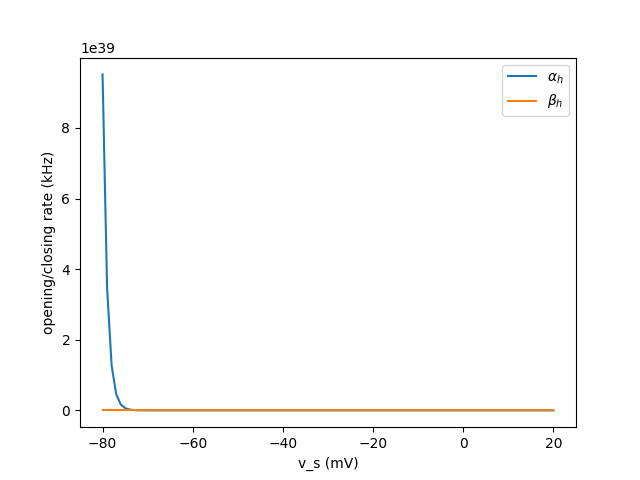
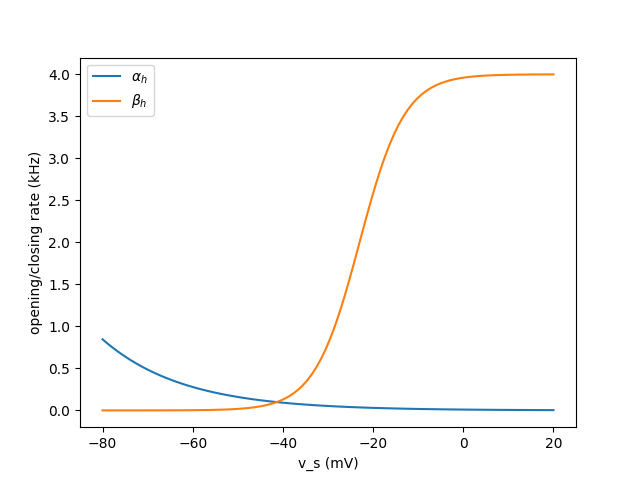
ah  = 0.128*(exp(17.0 - v_s/mV)/18.0) / ms : Hz
bh  = 4.0 /( 1.0 + (exp((40 - v_s/mV)/5.0)) ) / ms : Hz

a_s = 1.6/( 1.0 + (exp(-0.072*(v_d/mV - 65.0)))  )  / ms : Hz
b_s = 0.02*(v_d/mV - 51.1)/(exp((v_d/mV - 51.1)/5.0) -1.0) / ms : Hz



ac = (
    int(v_d <= 50*mV) *
    (exp((v_d/mV - 10.0)/11.0) - exp((v_d/mV - 6.5)/27.0)) / 18.975
    + int(v_d > 50*mV) * (2.0 * exp((6.5 - v_d/mV)/27.0))
) / ms : Hz


bc = ( int(v_d <= 50*mV) * (2.0 * exp((6.5 - v_d/mV)/27.0) - exp((v_d/mV - 10.0)/11.0) - exp((v_d/mV -  6.5)/27.0))/ 18.975
+ int(v_d > 50*mV) * 0) /ms : Hz

aq   =  clip(0.00002*Ca, 0, 0.01)/ms: Hz
bq   = 0.001/ms : Hz
chid = clip(Ca/250., 0, 1) : 1

#soma dynamics
dh/dt= ah - (ah+bh)* h: 1
dn/dt= an - (an+bn)* n: 1

# gating dynamics
ds/dt = (1-s)*a_s - s*b_s  : 1
dc/dt = (1-c)*ac - c*bc    : 1
dq/dt = (1-q)*aq - q*bq    : 1

#soma state

m_inf = 1.0/(1.0 + exp(-(v_s/mV + 30.0)/9.0)) : 1
h_inf = 1.0/(1.0 + exp((v_s/mV + 53.0)/7.0)) : 1
# tau_h = 1.0/(exp((v_s/mV+46.0)/20.0) + exp(-(v_s/mV+238)/20.0))*ms : second
n_inf = 1.0/(1.0 + exp(-(v_s/mV + 30.0)/10.0)) : 1
# tau_n = 1.0/(exp((v_s/mV+35.0)/40.0) + exp(-(v_s/mV-40.0)/50.0))*ms : second


# dh/dt = (h_inf - h)/tau_h : 1
# dn_s/dt = (n_inf - n_s)/tau_n : 1


C_s      : farad/meter**2
C_d      : farad/meter**2
I_s      : amp/meter**2
I_d      : amp/meter**2
g_Na     : siemens/meter**2
E_Na     : volt
g_Kdr    : siemens/meter**2
E_K      : volt
g_L      : siemens/meter**2
E_L      : volt
g_Ca     : siemens/meter**2
E_Ca     : volt
g_Kahp   : siemens/meter**2
g_Abeta  : siemens/meter**2
E_Abeta  : volt
g_c      : siemens/meter**2
g_KC     : siemens/meter**2
p        : 1

'''



neuron = NeuronGroup(1, model=eqs ,threshold='m_inf > 0.5',reset=None, method='exponential_euler',refractory='2*ms')
neuron.set_states(Parameters)
# for name, val in Parameters.items():
#        setattr(neuron, name, val)

# initials
neuron.v_s = -65 * mV
neuron.v_d = -65 * mV
neuron.h = 0.
neuron.q = 0.
neuron.n = 0.
neuron.Ca = 300.
neuron.s = 0.
neuron.c = 0.

# record & run

#M= StateMonitor(pyr_model, ['Vs','Vd','Cad','ILs',"INa",'ICad','IK_ahp','IK_C','ILd'], record=True)
M = StateMonitor(neuron, ['v_s', 'v_d', 'Ca', 'q','ILs','INa', 'IK_DR', 'ILd','ICad','IK_ahp','IK_C','I_Ca','h','n', 's','c','chid','ac','bc','ah'], record=True)
run(200 * ms)
print(neuron.g_c)

# plot
import matplotlib.pyplot as plt

figure(figsize=(12, 4))
plot(M.t/ms, M.ILd[0]/mV, label='ILd')
plot(M.t/ms, M.ICad[0]/mV, label='ICad')
plot(M.t/ms, M.IK_ahp[0]/mV, label='IK_ahp')
plot(M.t/ms, M.IK_C[0]/mV, label='IK_C')
plot(M.t/ms, M.ILs[0]/mV, label='ILs')
plot(M.t/ms, M.ILd[0]/mV, label='ILd')
plot(M.t/ms, M.INa[0]/mV, label='INa')
plot(M.t/ms, M.IK_DR[0]/mV, label='IK_DR')
legend()
xlabel('Time (ms)')
ylabel('Current (mV)')
show()

# 1. Voltage plot (choose v_s or v_d)
plt.figure(figsize=(7, 4))
plt.plot(M.t / ms, M.v_s[0] / mV, label='V_s (mV)')
#for dendrite: plt.plot(M.t/ms, M.v_d[0]/mV, label='V_d (mV)')
plt.xlabel('Time (ms)')
plt.ylabel('Voltage (mV)')
plt.title('Somatic Input')
plt.legend()
plt.tight_layout()
plt.show()

# 2. Ca and q plot (share axis, different units)
plt.figure(figsize=(7, 4))
plt.plot(M.t / ms, M.Ca[0], label='Ca (Ca units)')
# plt.plot(M.t / ms, M.q[0], label='q (AHP gating)')
plt.xlabel('Time (ms)')
plt.ylabel('Value')
plt.title('Ca and q on somatic input')
plt.legend()
plt.tight_layout()
plt.show()


plt.figure(figsize=(7, 4))
plot(M.t/ms, M.h[0]/mV, label='h')
plot(M.t/ms, M.q[0]/mV, label='q')
plot(M.t/ms, M.s[0]/mV, label='s')
plot(M.t/ms, M.n[0]/mV, label='n')
plt.xlabel('Time (ms)')
plt.ylabel('Value')
plt.legend()
plt.tight_layout()
plt.show()

plt.figure(figsize=(7, 4))
plot(M.t/ms, M.c[0]/mV, label='c')
plt.xlabel('Time (ms)')
plt.ylabel('Value')
plt.legend()
plt.tight_layout()
plt.show()

plt.figure(figsize=(7, 4))
plot(M.v_d[0]/mV, M.ac[0], label='ac')
plot(M.v_d[0]/mV, M.bc[0], label='bc')
plt.xlabel('voltage)')
plt.ylabel('value')
plt.legend()
plt.tight_layout()
plt.show()

plt.figure(figsize=(7, 4))
plot(M.Ca[0], M.chid[0], label='chid')
plt.xlabel('Value')
plt.ylabel('Ca')
plt.legend()
plt.tight_layout()
plt.show()

plt.figure(figsize=(7, 4))
plot(M.v_s[0]/mV, M.ah[0], label='ah')
plt.xlabel('voltage')
plt.ylabel('value')
plt.legend()
plt.tight_layout()
plt.show()

What you have aready tried

So I’ve tried to plot several values to identify the problem.

Expected output (if relevant)

the expected output is figure 2 page 8 from the paper

Actual output (if relevant)

figures about somatic voltage , Ca and q

Full traceback of error (if relevant)

From what I’ve plotted i believe that the problem is isolated to (ac),( bc) or potentialy (ah). Could be wrong tho

[mstimberg]

Hi @imlittledove. I did not go through everything in detail, but I think the rate equations for your gating variables are wrong (at least for ah). For complex models like this, I’d recommend to first make sure that all the equations that are a function of v (or in your case v_s or v_d) are correct and give the expected results, This approach here can be useful: How to plot functions — Brian 2 0.0.post128 documentation
When I do this for ah and bh from your equations, I get:

which indicates at least a problem for ah, it shouldn’t go that high in the physiological range. For comparison, here’s the corresponding plot from https://brian2.readthedocs.io/en/stable/examples/COBAHH.html:

Note that the equations are basically identical in both cases, but your equations do not shift the membrane potential by 63mV. Could it be that your equations assume a membrane potential convention where 0mV is the resting potential of the cell?

[imlittledove]

How would they assume a membrane potential on 0mV tho if on the equation the only v-value is v_s?
Can you think of anything that might lead the model to assume that?

Also about the equations I’m 99% sure they are correct based on the paper’s indications but for that i could check again.

[mstimberg]

Hi again. The equations you are using are meant for v_s and v_d relative to the resting potential, i.e. 0mV means “0mV above the resting potential” or something like -65mV. This is why your E_L is 0mV instead of around -65mV, E_Na is at 115mV instead of being at 50mV, etc. This is not a problem – mathematically you can replace v by v+65mV or the other way round everywhere, and the results are the same. You just have to be aware of it when you are interpreting the results, adding new equations, or when you are initializing variables. I actually did not take this into account when I plotted the functions above, since for your code I should have used a range from -15mV to 85mV for the equivalent of -80mV to 20mV (but it would still look very wrong).
Related to this, there is a minor mistake in your code, you probably do not want to initialize v_s and v_d to -65mV because this means -65mV below resting value, i.e. something like -130mV.
But more importantly, there is a mistake in the equation for ah, it should be exp((.../)18.0) instead of exp(....)/18.0, i.e. the division by 18 should be inside the argument of exp. There might be similar mistakes elsewhere, I’d use the approach mentioned above to verify that all opening/closing rates are doing what they are expected to do.

[imlittledove]

Thank you I’ll check what you said and post back tomorrow with new information after I’ve checked everything.

[imlittledove]

Hello! So i solve the problem and i wanted to share for whoever may come across the same problem. The problem was with the equations but not like what you suggested. The equations had completely wrong values, and my parameters that i found also had some wrong values. So I’m attaching here the correct code along with the paper for the corrected equations. Again thanks for the help!

#%%
from brian2 import *
import matplotlib.pyplot as plt
start_scope()

defaultclock.dt = 0.05 * ms

Parameters = {
    'C_s': 3 * uF / cm ** 2,
    'C_d': 3 * uF / cm ** 2,
    'I_s': 0.75 * uA/ cm ** 2,
    'I_d': 0 * uA/ cm ** 2 ,
    'v_s': -65*mV,
    'v_d': -65*mV,
    'g_Na': 30 * msiemens / cm ** 2,
    'E_Na': 60 * mV,
    'g_Kdr': 15 * msiemens / cm ** 2,
    'E_K': -75 * mV,
    'g_L': 0.1 * msiemens / cm ** 2,  # leak
    'E_L': -60 * mV,
    'g_Ca': 7 * msiemens / cm ** 2,
    'E_Ca': 80 * mV,
    'g_Kahp': 0.8 * msiemens / cm ** 2,
    'g_KC': 15 * msiemens / cm ** 2,
    'g_Abeta': 0 * msiemens / cm ** 2,
    'E_Abeta': -65 * mV,
    'g_c': 1.75 * usiemens / cm ** 2,
    'p': 0.5,

}

eqs = '''
#membrane potential
#soma:
dv_s/dt=(- ILs -INa - IK_DR + (g_c/p) * (v_d-v_s) + (I_s/p))/C_s: volt

#dendrite:
dv_d/dt = ( - ILd - ICad - IK_ahp - IK_C + (g_c/(1.0-p)) * (v_s - v_d) -(g_Abeta * (v_d - E_Abeta)) + I_d/(1.0-p))/C_d: volt

ILs   = g_L * (v_s - E_L) : amp/meter**2
INa   = g_Na *m_inf*m_inf * h * (v_s - E_Na) :amp/meter**2
IK_DR = g_Kdr * n * (v_s - E_K) :amp/meter**2

ILd    = g_L * (v_d - E_L) :amp/meter**2
ICad   = g_Ca *s*s* (v_d - E_Ca) :amp/meter**2
IK_ahp = g_Kahp * q * (v_d - E_K) :amp/meter**2
IK_C   = g_KC *c* chid * (v_d - E_K) :amp/meter**2


# [ Ca ]
I_Ca = g_Ca * s**2 * (v_d - E_Ca) : amp/meter**2
dCa/dt = ( -0.13 * (I_Ca / (uA/cm**2)) - 0.075 * Ca ) / ms : 1

# Appendix
am  = 0.32*(-49.9 - v_s/mV)/(exp((-46.9 - v_s/mV)/4.0) - 1.0) / ms : Hz
bm  = 0.28*(v_s/mV + 19.9)/(exp((v_s/mV + 19.9)/5.0) - 1.0) / ms : Hz

an  = 0.016*(-24.9 - v_s/mV)/ (exp((-24.9 - v_s/mV)/5.0) -1.0) / ms : Hz
bn  = 0.25*exp(-1.0 - 0.025 *v_s/mV)/ms: Hz

ah  = 0.128*exp((-43.0 - v_s/mV)/18.0) / ms : Hz
bh  = 4.0 /( 1.0 + exp((-20.0 - v_s/mV)/5.0) ) / ms : Hz

a_s = 1.6/( 1.0 + exp(-0.072*(v_d/mV - 5.0))  )  / ms : Hz
b_s = 0.02*(v_d/mV +8.9)/(exp((v_d/mV +8.9)/5.0) - 1.0) / ms : Hz


ac = (
    int(v_d <= 50*mV) *
    (exp((v_d/mV +50.0)/11.0) - exp((v_d/mV +53.5)/27.0)) / 18.975
    + int(v_d > 50*mV) * (2.0 * exp((-53.5 - v_d/mV)/27.0))
) / ms : Hz


bc = ( int(v_d <= 50*mV) * (2.0 * exp((-53.5 - v_d/mV)/27.0) - exp((v_d/mV + 50.0)/11.0) - exp((v_d/mV +53.5)/27.0))/ 18.975
+ int(v_d > 50*mV) * 0) /ms : Hz

aq   =  clip(0.00002*Ca, 0, 0.01)/ms: Hz
bq   = 0.001/ms : Hz
chid = clip(Ca/250., 0, 1) : 1

#soma dynamics
dh/dt= ah - (ah+bh)* h: 1
dn/dt= an - (an+bn)* n: 1

# gating dynamics
ds/dt = (1-s)*a_s - s*b_s  : 1
dc/dt = (1-c)*ac - c*bc    : 1
dq/dt = (1-q)*aq - q*bq    : 1

#soma state

m_inf = 1.0/(1.0 + exp(-(v_s/mV + 30.0)/9.0)) : 1
h_inf = 1.0/(1.0 + exp((v_s/mV + 53.0)/7.0)) : 1
# tau_h = 1.0/(exp((v_s/mV+46.0)/20.0) + exp(-(v_s/mV+238)/20.0))*ms : second
n_inf = 1.0/(1.0 + exp(-(v_s/mV + 30.0)/10.0)) : 1
# tau_n = 1.0/(exp((v_s/mV+35.0)/40.0) + exp(-(v_s/mV-40.0)/50.0))*ms : second



C_s      : farad/meter**2
C_d      : farad/meter**2
I_s      : amp/meter**2
I_d      : amp/meter**2
g_Na     : siemens/meter**2
E_Na     : volt
g_Kdr    : siemens/meter**2
E_K      : volt
g_L      : siemens/meter**2
E_L      : volt
g_Ca     : siemens/meter**2
E_Ca     : volt
g_Kahp   : siemens/meter**2
g_Abeta  : siemens/meter**2
E_Abeta  : volt
g_c      : siemens/meter**2
g_KC     : siemens/meter**2
p        : 1

'''


neuron = NeuronGroup(1, model=eqs ,threshold='m_inf > 0.5',reset=None, method='exponential_euler',refractory='2*ms')
neuron.set_states(Parameters)
# for name, val in Parameters.items():
#        setattr(neuron, name, val)

# initials
neuron.v_s = -60 * mV
neuron.v_d = -60 * mV
neuron.h = 0.999
neuron.q = 0.01
neuron.n = 0.0001
neuron.Ca = 0.2
neuron.s = 0.009
neuron.c = 0.007

# record & run

#M= StateMonitor(pyr_model, ['Vs','Vd','Cad','ILs',"INa",'ICad','IK_ahp','IK_C','ILd'], record=True)
M = StateMonitor(neuron, ['v_s', 'v_d', 'Ca', 'q','ILs','INa', 'IK_DR', 'ILd','ICad','IK_ahp','IK_C','I_Ca','h','n', 's','c','chid','ac','bc','ah'], record=True)
run(200 * ms)
# print(neuron.g_c)

# plot
import matplotlib.pyplot as plt

# 1. Voltage plot (choose v_s or v_d)
plt.figure(figsize=(7, 4))
plt.plot(M.t / ms, M.v_s[0] / mV, label='V_s (mV)')
#for dendrite: plt.plot(M.t/ms, M.v_d[0]/mV, label='V_d (mV)')
plt.xlabel('Time (ms)')
plt.ylabel('Voltage (mV)')
plt.title('Somatic Input')
plt.legend()
plt.tight_layout()
plt.show()


# 2. Ca and q plot (share axis, different units)
plt.figure(figsize=(7, 4))
plt.plot(M.t / ms, M.Ca[0], label='Ca (Ca units)')
plot(M.t/ms, M.q[0]/mV, label='q')
# plt.plot(M.t / ms, M.q[0], label='q (AHP gating)')
plt.xlabel('Time (ms)')
plt.ylabel('Value')
plt.title('Ca and q on somatic input')
plt.legend()
plt.tight_layout()
plt.show()


figure(figsize=(12, 4))
plot(M.t/ms, M.ILd[0]/mV, label='ILd')
plot(M.t/ms, M.ICad[0]/mV, label='ICad')
plot(M.t/ms, M.IK_ahp[0]/mV, label='IK_ahp')
plot(M.t/ms, M.IK_C[0]/mV, label='IK_C')
plot(M.t/ms, M.ILs[0]/mV, label='ILs')
plot(M.t/ms, M.ILd[0]/mV, label='ILd')
plot(M.t/ms, M.INa[0]/mV, label='INa')
plot(M.t/ms, M.IK_DR[0]/mV, label='IK_DR')
legend()
xlabel('Time (ms)')
ylabel('Current (mV)')
show()


plt.figure(figsize=(7, 4))
plot(M.t/ms, M.h[0]/mV, label='h')
plot(M.t/ms, M.s[0]/mV, label='s')
plot(M.t/ms, M.n[0]/mV, label='n')
plt.xlabel('Time (ms)')
plt.ylabel('Value')
plt.legend()
plt.tight_layout()
plt.show()

plt.figure(figsize=(7, 4))
plot(M.t/ms, M.c[0]/mV, label='c')
plt.xlabel('Time (ms)')
plt.ylabel('Value')
plt.legend()
plt.tight_layout()
plt.show()

plt.figure(figsize=(7, 4))
plot(M.v_d[0]/mV, M.ac[0], label='ac')
plot(M.v_d[0]/mV, M.bc[0], label='bc')
plt.xlabel('voltage)')
plt.ylabel('value')
plt.legend()
plt.tight_layout()
plt.show()

plt.figure(figsize=(7, 4))
plot(M.Ca[0], M.chid[0], label='chid')
plt.xlabel('Value')
plt.ylabel('Ca')
plt.legend()
plt.tight_layout()
plt.show()

plt.figure(figsize=(7, 4))
plot(M.v_s[0]/mV, M.ah[0], label='ah')
plt.xlabel('voltage')
plt.ylabel('value')
plt.legend()
plt.tight_layout()
plt.show()

Here i found the correct version of the equations and parameters:

ModelDB: Show Model

[mstimberg]

Hi @imlittledove, thanks for sharing the code, happy to hear that it works now! From a cursory look these seem to be still basically the same equations/values, just shifted as I explained earlier. E.g. E_L is now -60mV instead of 0mV earlier,
and e.g. your equation for ah is now

ah  = 0.128*exp((-43.0 - v_s/mV)/18.0) / ms : Hz

In the old code the membrane potential, let’s call it v_s_old, represented v_s + 60mV, therefore this equation is

ah  = 0.128*exp((-43.0 - (v_s_old /mV - 60))/18.0) / ms : Hz

==>

ah  = 0.128*exp((-43.0 + 60 - v_s_old /mV)/18.0) / ms : Hz

==>

ah  = 0.128*exp((17 - v_s_old /mV)/18.0) / ms : Hz

which is the same equation has you had in the code posted earlier (except for the incorrect position of /18.0 of course).